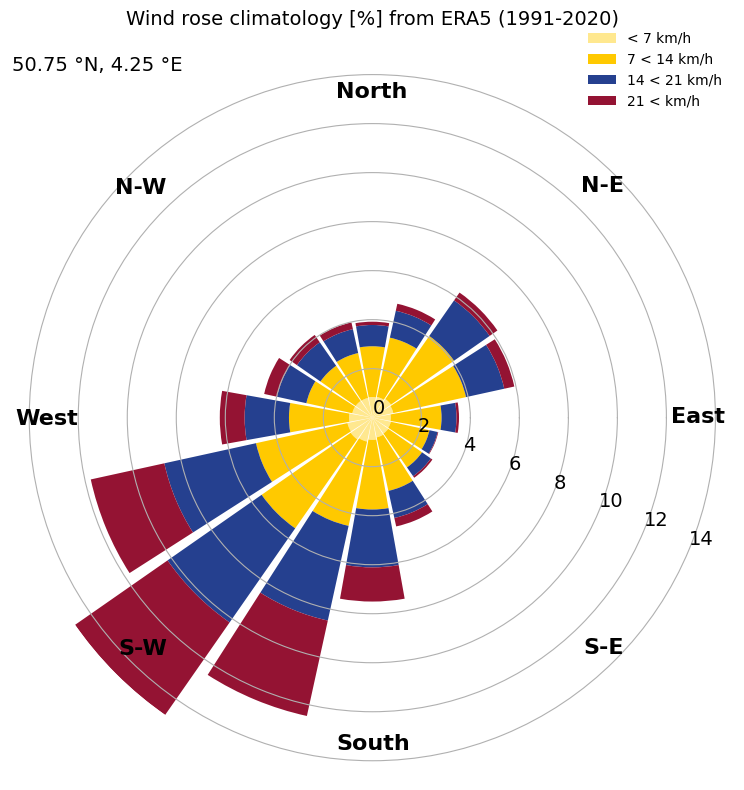
Calculate the hourly climatological wind from ERA5#
This notebook demonstrates how to retrieve, process, and plot the data displayed in the ERA Explorer
==> For further training materials, consider the Copernicus Climate Change Service (C3S) data tutorials
In this example we will be using earthkit to retrieve the data and standard Python packages to process and plot it.
import numpy as np
import pandas as pd
import matplotlib.pyplot as plt
import calendar
import earthkit.data
If you want to run this code yourself, make sure to get a CDS API key from the CDS website.
Following the guidance there, you’ll then need to set up your local .cdsapirc to be able to authenticate with the CDS and download data. Then, you will be able to customise the date ranges, variables, and much more!
This is the latitude/longitude that we will extract the nearest grid cell from. You can change these to plot different locations. You can see the currently used ones in the ERA Explorer URL. In this example we are plotting data at the gridpoint closest to Brussels, Belgium.
lat = 50.86
lng = 4.35
This is the variable we are getting from the ERA dataset, and the time period
variable = "10m_u_component_of_wind"
date_range = ["1991-01-01", "2020-12-31"]
To calculate wind direction we need the v-component of the wind as well
variable2 = "10m_v_component_of_wind"
For convenience, we make a function to handle the data retrieval:
def retrieve_data(variable, date_range, lat, lng):
    # Define the dataset and request parameters
    dataset = "reanalysis-era5-single-levels-timeseries"
    request = {
        "variable": [
        variable,  # Variable to retrieve
        ],
        "date": date_range,  # Date range for the data
        "location": {"longitude": lng, "latitude": lat},  # Location coordinates
        "data_format": "netcdf"  # Format of the retrieved data
    }

    # Use "earthkit" to retrieve the data
    ekds = earthkit.data.from_source(
        "cds", dataset, request
    ).to_xarray()

    return ekds
Get the data. This will download a NetCDF file
data = retrieve_data(variable, date_range, lat, lng)
To calculate relative humidity we need dewpoint temperature as well
data2 = retrieve_data(variable2, date_range, lat, lng)
And let’s make some bespoke functions to process the data. Each one is described with a “””docstring”””
# Define a function to bin angles into 45-degree chunks with an offset of -22.5 degrees
def bin_angle(angle, nbins=8):
    """
    Bin an angle into one of the specified number of bins.

    Parameters:
        angle (float): The angle in degrees to be binned.
        nbins (int): The number of bins to divide the 360 degrees into. Default is 8.

    Returns:
        str: The label of the bin into which the angle falls,
             formatted as 'start to end' degrees.

    Example:
        >>> bin_angle(45, 8)
        '22.5 to 67.5'
    """
    angle = angle % 360
    width = 360 / nbins
    offset = width / 2
    adjusted_angle = (angle + offset) % 360
    bin_index = int(np.floor(adjusted_angle / width))
    bin_labels = [
        '{:.1f} to {:.1f}'.format(i * width - offset, i * width + offset)
        for i in range(nbins)
    ]
    return bin_labels[bin_index]


# Define a function to calculate wind magnitude and convert to km/h
def calculate_magnitude(u, v):
    """
    Calculate the magnitude of a vector given its u and v components.

    Parameters:
        u (array-like): The u component of the vector.
        v (array-like): The v component of the vector.

    Returns:
        numpy.ndarray: The magnitude of the vector.
    """
    metres_per_sec_to_km_h = 3.6
    magnitude = np.sqrt(u**2 + v**2) * metres_per_sec_to_km_h
    return magnitude


# Define a function to bin magnitudes into categories
def bin_magnitude(magnitude, cutoffs):
    """
    Categorizes a given magnitude into a bin based on provided cutoff values.

    Parameters:
        magnitude (float): The magnitude value to be categorized.
        cutoffs (list of int): A list of cutoff values that define the bins.
                               The list should have exactly 4 elements.

    Returns:
        str: A string representing the bin in which the magnitude falls.
    """
    if magnitude < cutoffs[1]:
        if cutoffs[0] == 0:
            return "< {:d}".format(cutoffs[1])
        else:
            return "{:d} < {:d}".format(cutoffs[0], cutoffs[1])
    elif magnitude < cutoffs[2]:
        return "{:d} < {:d}".format(cutoffs[1], cutoffs[2])
    elif magnitude < cutoffs[3]:
        return "{:d} < {:d}".format(cutoffs[2], cutoffs[3])
    else:
        return "{:d} <".format(cutoffs[3])


# Make a function to compute the wind climatology
def windMonthlyClimatology():
    """
    Calculate the monthly climatology of wind direction and magnitude.

    This function reads wind data from two NetCDF files, calculates the wind direction
    angle and magnitude, bins the data into specified angle and magnitude bins,
    and returns the percentage of occurrences in each bin.

    Returns:
        bin_percentages (pd.DataFrame): A DataFrame containing the percentage of
                                        occurrences in each angle and magnitude bin.
        angle_bins (list): A list of angle bin labels.
        cutoff_labels (list): A list of magnitude bin labels.
    """
    # Load data
    data_u10_pt = data.u10
    data_v10_pt = data2.v10

    # Convert xarray DataArrays to pandas Series
    u_series = data_u10_pt.to_series()
    v_series = data_v10_pt.to_series()

    # Calculate wind direction angle
    angle = np.arctan2(-u_series, -v_series) * (180 / np.pi)

    # Create a DataFrame
    df = pd.DataFrame({
        'u': u_series,
        'v': v_series,
        'Time': u_series.index,
        'Angle': angle
    })
    df.sort_values('Time', inplace=True)

    # Add wind magnitude to DataFrame
    df['Magnitude'] = calculate_magnitude(df['u'], df['v'])

    # Bin angles and magnitudes
    df['Angle Bin'] = df['Angle'].apply(lambda x: bin_angle(x, 16))
    nearest_even = int(np.round(df['Magnitude'].median() / 2) * 2)
    cutoffs = [0, int(nearest_even / 2), nearest_even, int(nearest_even * 1.5)]
    df['Magnitude Bin'] = df['Magnitude'].apply(lambda x: bin_magnitude(x, cutoffs))

    # Define bins
    angle_bins = [bin_angle(i * 360 / 16, 16) for i in range(16)]
    cutoff_labels = [bin_magnitude(cutoffs[i], cutoffs) for i in range(len(cutoffs))]

    # Count occurrences in bins
    bin_counts = (
        df.groupby(["Angle Bin", "Magnitude Bin"]).size().unstack(fill_value=0)
    )
    bin_counts = bin_counts.reindex(index=angle_bins,
                                    columns=cutoff_labels, fill_value=0)

    # Convert to percentages
    bin_percentages = 100 * bin_counts / bin_counts.sum(axis=1).sum(axis=0)

    # Sort and reindex
    bin_percentages.index = pd.CategoricalIndex(
        bin_percentages.index, categories=angle_bins, ordered=True
    )
    bin_percentages.sort_index(inplace=True)
    bin_percentages = bin_percentages.reindex(columns=cutoff_labels)

    # Get the actual lat/lon used
    nearest_lat = data_u10_pt.latitude.values
    nearest_lng = data_u10_pt.longitude.values

    return bin_percentages, angle_bins, cutoff_labels, nearest_lat, nearest_lng


# Call our function
bin_percentages, angle_bins, cutoff_labels, \
    nearest_lat, nearest_lng = windMonthlyClimatology()
And finally, let’s set up the plot nicely. This can easily be customised, but for now we do something similar to ERA Explorer
# Determine the suffix for latitude (N/S) and longitude (E/W) based on their signs
latSuffix = 'N' if nearest_lat > 0 else 'S'
lngSuffix = 'E' if nearest_lng > 0 else 'W'

# Generate a list of abbreviated month names (Jan, Feb, etc.)
month_names = [calendar.month_abbr[i] for i in range(1, 13)]

# Define directional labels for the wind rose (e.g., North, North-East, etc.)
direction_labels = ['North', 'N-E', 'East', 'S-E', 'South', 'S-W', 'West', 'N-W']

# Number of bins for the histogram
nbins = bin_percentages.shape[0]

# Calculate the width of each bin and bin centers (in radians) for polar plot
width = 0.9 * 2 * np.pi / nbins
angles = np.linspace(0, 2 * np.pi, nbins, endpoint=False) - np.pi / 2

# Calculate cumulative percentages and set y-axis limit
cumul_bin_percentages = bin_percentages.sum(axis=1).values
ylim1 = max(cumul_bin_percentages)

# Define colors for stacked bars
colors = ['#FFE88F', '#FFC900', '#25408F', '#941333']

# Create a polar plot
fig, ax = plt.subplots(figsize=(8, 8), subplot_kw={'projection': 'polar'})

# Configure polar plot appearance
ax.set_frame_on(False)
ax.set_theta_direction(-1)
ax.set_ylim(0, ylim1)
ax.set_xticks([])
ax.set_yticks(range(0, int(max(cumul_bin_percentages)) + 2, 2))
ax.tick_params(axis='y', labelsize=14)

# Add directional labels and shade alternate segments
for index, angle in enumerate(np.arange(0, 360, 45)):
    mid_angle = np.deg2rad(angle)
    start_angle = mid_angle - np.deg2rad(width / 2)
    ax.text(start_angle - np.pi / 2, 0.9 * ylim1, direction_labels[index],
            ha='center', va='center', fontsize=16, fontweight='bold')

# Plot stacked bars for each bin
for i, col in enumerate(bin_percentages.columns):
    ax.bar(angles, bin_percentages[col], width=width,
           bottom=bin_percentages.iloc[:, :i].sum(axis=1),
           color=colors[i], linewidth=1, label=f'{cutoff_labels[i]} km/h')

# Add legend and title
ax.legend(loc='upper right', bbox_to_anchor=(1, 1.05), framealpha=0)
plt.title(f'Wind rose climatology [%] from ERA5 '
          f'({date_range[0][:4]}-{date_range[1][:4]})\n', fontsize=14)

# Add latitude and longitude text
label = (
    f'{abs(nearest_lat):.2f} °{latSuffix:s}, '
    f'{abs(nearest_lng):.2f} °{lngSuffix:s}'
)
fig.text(0.05, 0.9, label,
         ha='left', va='bottom', fontsize=14)

# Adjust layout and render the plot
plt.tight_layout()
plt.show()