Calculate the monthly climatological temperature from ERA5#
This notebook demonstrates how to retrieve, process, and plot the data displayed in the ERA Explorer
==> For further training materials, consider the Copernicus Climate Change Service (C3S) data tutorials
In this example we will be using earthkit to retrieve the data and standard Python packages to process and plot it.
import pandas as pd
import matplotlib.pyplot as plt
import calendar
import earthkit.data
If you want to run this code yourself, make sure to get a CDS API key from the CDS website.
Following the guidance there, you’ll then need to set up your local .cdsapirc to be able to authenticate with the CDS and download data. Then, you will be able to customise the date ranges, variables, and much more!
This is the latitude/longitude that we will extract the nearest grid cell from. You can change these to plot different locations. You can see the currently used ones in the ERA Explorer URL. In this example we are plotting data at the gridpoint closest to Brussels, Belgium.
lat = 50.86
lng = 4.35
This is the variable we are getting from the ERA dataset, and the time period
variable = "2m_temperature"
date_range = ["1991-01-01", "2020-12-31"]
For convenience, we make a function to handle the data retrieval:
def retrieve_data(variable, date_range, lat, lng):
    # Define the dataset and request parameters
    dataset = "reanalysis-era5-single-levels-timeseries"
    request = {
        "variable": [
        variable,  # Variable to retrieve
        ],
        "date": date_range,  # Date range for the data
        "location": {"longitude": lng, "latitude": lat},  # Location coordinates
        "data_format": "netcdf"  # Format of the retrieved data
    }

    # Use "earthkit" to retrieve the data
    ekds = earthkit.data.from_source(
        "cds", dataset, request
    ).to_xarray()

    return ekds
Get the data. This will download a NetCDF file
data = retrieve_data(variable, date_range, lat, lng)
And let’s make some bespoke functions to process the data. Each one is described with a “””docstring”””
# Make a function to compute the monthly temperature climatology
def temperatureMonthlyClimatology():
    """
    Processes temperature data to calculate monthly climatology and thresholds.

    This function reads temperature data from a NetCDF file, processes it to calculate
    daily minimum and maximum temperatures, and then computes monthly climatology
    statistics. It also calculates the percentage of frost days, tropical nights, and
    summer days per month over a 30-year period.

    Returns:
        tuple: A tuple containing the following elements:
            - monthly_climatology (pd.DataFrame): Climatological averages for daily
              minimum and maximum temperatures per month, converted to Celsius.
            - frost_day_climatology (pd.Series): Average percentage of frost days
              per month.
            - tropical_night_climatology (pd.Series): Average percentage of tropical
              nights per month.
            - summer_day_climatology (pd.Series): Average percentage of summer days
              per month.
    """

    data_t2m_pt = data.t2m

    # Convert the time coordinate to a pandas datetime index
    time_index = pd.to_datetime(data_t2m_pt.valid_time.values)

    # Create a DataFrame for easier manipulation
    df = pd.DataFrame(data_t2m_pt.values, index=time_index, columns=['t2m'])

    # Resample to find daily minimum and maximum
    daily_min = df.resample('D').min()
    daily_max = df.resample('D').max()

    # Combine the daily min and max into a single DataFrame
    daily_stats = pd.DataFrame({
        'daily_min': daily_min['t2m'],
        'daily_max': daily_max['t2m']
    })

    # Define the frost night threshold (e.g., 0°C in Kelvin)
    frostDayThreshold = 0 + 273.15
    tropicalNightThreshold = 20 + 273.15
    summerDayThreshold = 25 + 273.15

    # Check if the daily minimum is below the threshold
    daily_min['frost_day'] = daily_min['t2m'] < frostDayThreshold
    daily_min['tropical_night'] = daily_min['t2m'] > tropicalNightThreshold
    daily_max['summer_day'] = daily_max['t2m'] > summerDayThreshold

    # Count the number of frost days (days below the threshold) per month
    frost_day_counts = daily_min.resample('ME').sum()['frost_day']
    tropical_night_counts = daily_min.resample('ME').sum()['tropical_night']
    summer_day_counts = daily_max.resample('ME').sum()['summer_day']

    # Count the total number of days per month
    total_days_per_month = daily_min.resample('ME').size()

    # Calculate the percentage of frost nights per month
    frost_day_pc = (frost_day_counts / total_days_per_month) * 100
    tropical_night_pc = (tropical_night_counts / total_days_per_month) * 100
    summer_day_pc = (summer_day_counts / total_days_per_month) * 100

    # Convert the index to month
    frost_day_pc.index = frost_day_pc.index.month
    tropical_night_pc.index = tropical_night_pc.index.month
    summer_day_pc.index = summer_day_pc.index.month

    # Group by month and calculate the average percentage over the 30-year period
    frost_day_climatology = frost_day_pc.groupby(frost_day_pc.index).mean()
    tropical_night_climatology = tropical_night_pc.groupby(tropical_night_pc.index).mean()
    summer_day_climatology = summer_day_pc.groupby(summer_day_pc.index).mean()

    # Extract the month from DateTimeIndex
    daily_stats['month'] = daily_stats.index.month

    # Group by month and calculate climatological averages for daily min and max
    grouped_by_month = daily_stats.groupby('month')
    monthly_climatology = grouped_by_month.mean() - 273.15  # Convert to Celsius

    # Get the actual lat/lon used
    nearest_lat = data_t2m_pt.latitude.values
    nearest_lng = data_t2m_pt.longitude.values

    return monthly_climatology, frost_day_climatology, \
           tropical_night_climatology, summer_day_climatology, \
           nearest_lat, nearest_lng

# Call our function
clim, frost_clim, tropical_clim, summer_clim, \
  nearest_lat, nearest_lng = temperatureMonthlyClimatology()
And finally, let’s set up the plot nicely. This can easily be customised, but for now we do something similar to ERA Explorer
# Set line width and marker properties for the plot
lw = 2 # Line width for potential lines in the plot
marker = 'o' # Marker style for potential points
markersize = 4 # Marker size
# Determine the suffix for latitude (N/S) and longitude (E/W) based on their signs
latSuffix = 'N' if nearest_lat > 0 else 'S'
lngSuffix = 'E' if nearest_lng > 0 else 'W'
# Create a new figure with a specified size
plt.figure(figsize=(8, 6))
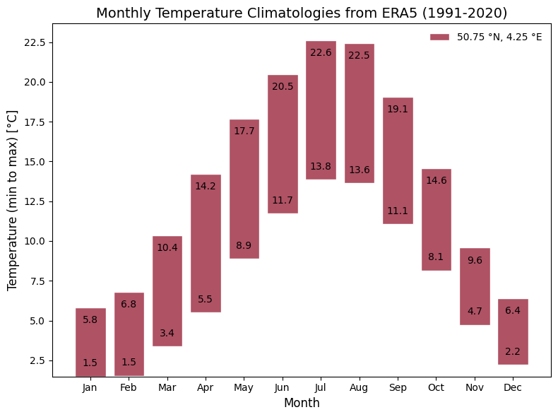
# Plot the data as a bar chart
bars = plt.bar(
clim.index, # X-axis values (months)
clim['daily_max'] - clim['daily_min'], # Heights of the bars (temperature range)
bottom=clim['daily_min'], # Base of each bar (minimum temperature)
width=0.8, # Width of the bars
color='#AF5264', # Fill color of the bars
edgecolor='white', # Edge color of the bars
label=(
f'{abs(nearest_lat):.2f} °{latSuffix:s}, '
f'{abs(nearest_lng):.2f} °{lngSuffix:s}'
)
)
# Add labels to each bar (minimum and maximum temperature values)
for index, bar in enumerate(bars):
# Retrieve minimum temperature for the current month
daily_min = clim['daily_min'].iloc[index]
# Retrieve maximum temperature for the current month
daily_max = clim['daily_max'].iloc[index]
# Compute the x-coordinate for the text (center of the bar)
x = bar.get_x() + bar.get_width() / 2
# Add a label for the minimum temperature near the bottom of the bar
plt.text(
x, # X position (center of the bar)
bar.get_y() + 0.5, # Y position (slightly above the base of the bar)
f'{daily_min:.1f}', # Label text showing the minimum temperature
ha='center', # Center the text horizontally
va='bottom', # Align the text just above the bar's base
fontsize=10, # Font size of the text
color='black' # Text color
)
# Add a label for the maximum temperature near the top of the bar
plt.text(
x, # X position (center of the bar)
bar.get_height() + bar.get_y() - 0.5, # Y position (slightly below top)
f'{daily_max:.1f}', # Label text showing the maximum temperature
ha='center', # Center the text horizontally
va='top', # Align the text just below the bar's top
fontsize=10, # Font size of the text
color='black' # Text color
)
# Add legend to the plot with no background frame
plt.legend(framealpha=0)
# Customize x and y axis labels
plt.xlabel('Month', fontsize=12) # Label for the x-axis
plt.ylabel('Temperature (min to max) [°C]', fontsize=12) # Label for the y-axis
# Set x-axis ticks to correspond to month indices and display month abbreviations
plt.xticks(ticks=clim.index, labels=[calendar.month_abbr[i] for i in clim.index])
# Add a title with the specified date range and custom font size
years = f'{date_range[0][:4]}-{date_range[1][:4]}'
plt.title(f'Monthly Temperature Climatologies from ERA5 ({years})', fontsize=14)
# Adjust layout to ensure all elements are properly displayed and do not overlap
plt.tight_layout()
# Display the final plot
plt.show()