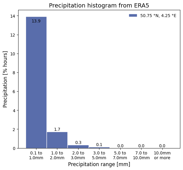
Calculate the histogram of hourly precipitation from ERA5

This notebook demonstrates how to retrieve, process, and plot the data displayed in the ERA Explorer

==> For further training materials, consider the Copernicus Climate Change Service (C3S) data tutorials

In this example we will be using earthkit to retrieve the data and standard Python packages to process and plot it.

import numpy as np
import pandas as pd
import matplotlib.pyplot as plt
import earthkit.data

If you want to run this code yourself, make sure to get a CDS API key from the CDS website.

Following the guidance there, you’ll then need to set up your local .cdsapirc to be able to authenticate with the CDS and download data. Then, you will be able to customise the date ranges, variables, and much more!

This is the latitude/longitude that we will extract the nearest grid cell from. You can change these to plot different locations. You can see the currently used ones in the ERA Explorer URL. In this example we are plotting data at the gridpoint closest to Brussels, Belgium.

lat = 50.86
lng = 4.35

This is the variable we are getting from the ERA dataset, and the time period

variable = "total_precipitation"
date_range = ["1991-01-01", "2020-12-31"]

For convenience, we make a function to handle the data retrieval:

def retrieve_data(variable, date_range, lat, lng):
    # Define the dataset and request parameters
    dataset = "reanalysis-era5-single-levels-timeseries"
    request = {
        "variable": [
        variable,  # Variable to retrieve
        ],
        "date": date_range,  # Date range for the data
        "location": {"longitude": lng, "latitude": lat},  # Location coordinates
        "data_format": "netcdf"  # Format of the retrieved data
    }

    # Use "earthkit" to retrieve the data
    ekds = earthkit.data.from_source(
        "cds", dataset, request
    ).to_xarray()

    return ekds

Get the data. This will download a NetCDF file

data = retrieve_data(variable, date_range, lat, lng)

And let’s make some bespoke functions to process the data. Each one is described with a “””docstring”””

# Make a function to compute the precipitation histogram
def precipHourlyHistogram():
    """
    Generates a histogram of hourly precipitation data.

    This function reads precipitation data from a NetCDF file,
    converts the time coordinate to a pandas datetime index,
    and creates a DataFrame for easier manipulation.
    It then resamples the data to hourly accumulations and computes
    a histogram with non-linear bins.
    The histogram values are converted to percentages, and the bin edges are
    converted to millimeters.

    Returns:
        tuple: A tuple containing:
            - hist_values (numpy.ndarray): The histogram values as percentages.
            - bin_edges (numpy.ndarray): The edges of the bins in millimeters.
    """

    data_tp_pt = data.tp

    # Convert the time coordinate to a pandas datetime index
    time_index = pd.to_datetime(data_tp_pt.valid_time.values)

    # Create a DataFrame for easier manipulation
    df = pd.DataFrame(data_tp_pt.values, index=time_index, columns=['tp'])

    # Count the total number of hours in the period
    total = df.resample('h').count().count().values[0]

    # Resample to hourly accumulations
    df_hourly = df.resample('h').sum()

    # Define non-linear bins for the histogram
    bins_nonlinear = np.array([0.0001, 0.001, 0.002, 0.003, 0.005, 0.007, 0.01, 100])

    # Put everything above the max in the last bin
    bins_nonlinear[-1] = 1e6

    # Compute the histogram
    hist_values, bin_edges = np.histogram(df_hourly['tp'], bins=bins_nonlinear)

    # Convert histogram values to percentage
    hist_values = 100 * hist_values / total
    
    # Convert bin edges to mm
    bin_edges = bin_edges * 1000

    # Get the actual lat/lon used
    nearest_lat = data_tp_pt.latitude.values
    nearest_lng = data_tp_pt.longitude.values

    return hist_values, bin_edges, nearest_lat, nearest_lng

hist_values, bin_edges, nearest_lat, nearest_lng = precipHourlyHistogram()

And finally, let’s set up the plot nicely. This can easily be customised, but for now we do something similar to ERA Explorer

# Determine suffix for latitude (N/S) and longitude (E/W) based on their sign
latSuffix = 'N' if nearest_lat > 0 else 'S'  # 'N' for +ve latitude, 'S' for -ve latitude
lngSuffix = 'E' if nearest_lng > 0 else 'W'  # 'E' for +ve longitude, 'W' for -ve longitude

# Get the maximum value of the histogram for scaling text labels
yMax = hist_values.max()

# Create x-axis tick labels as precipitation ranges
xtick_labels = [
    (
        f'{(bin_edges[i]):.1f} to\n{(bin_edges[i+1]):.1f}mm'
        if i < len(bin_edges) - 2
        else f'{(bin_edges[-2]):.1f}mm\nor more'
    )
    for i in range(len(bin_edges) - 1)
]

# Create a new figure with a specified size
plt.figure(figsize=(7, 6))

# Plot the histogram as a bar chart
bars = plt.bar(
    np.arange(len(hist_values)),  # X positions for bars
    hist_values,                 # Heights of the bars (histogram values)
    width=1,                     # Width of each bar
    color='#596DAB',             # Bar fill color
    label=(
        f'{abs(nearest_lat):.2f} °{latSuffix}, '
        f'{abs(nearest_lng):.2f} °{lngSuffix}'
    ),                           # Legend label
    edgecolor='white',           # Color of the bar edges
    clip_on=False                # Ensure bars are not clipped at the plot edges
)

# Add value labels on each bar
for index, bar in enumerate(bars):
    value = hist_values[index]  # Get the value of the current bar
    x = bar.get_x() + bar.get_width() / 2  # Center of the bar

    # Add the label text above or below the bar depending on its position
    plt.text(
        x,                                 # X position (center of the bar)
        bar.get_height() + bar.get_y() + 
        (-0.02 * yMax if index <= 0 else 0),  # Adjust Y position
        f'{value:.1f}',                    # Text label (formatted value)
        ha='center',                       # Horizontal alignment: center
        va=('bottom' if index > 0 else 'top'),  # Vertical alignment
        fontsize=10,                       # Font size of the text
        color='black'                      # Text color
    )

# Add a legend with a transparent background
plt.legend(framealpha=0)

# Set x-axis tick positions and labels
plt.xticks(
    np.arange(len(hist_values)),  # Positions for each tick
    xtick_labels                 # Labels for each tick
)

# Optional: Set y-axis limits
# plt.ylim(0, hist_values.max())

# Add labels to the x and y axes
plt.xlabel(
    'Precipitation range [mm]', 
    fontsize=12
)
plt.ylabel(
    "Precipitation [% hours]", 
    fontsize=12
)

# Add a title to the plot
plt.title(
    'Precipitation histogram from ERA5', 
    fontsize=14
)

# Optional: Adjust the layout to prevent overlapping elements
# plt.tight_layout()

# Display the plot
plt.show()