Calculate the daily climatological temperature from ERA5#
This notebook demonstrates how to retrieve, process, and plot the data displayed in the ERA Explorer
==> For further training materials, consider the Copernicus Climate Change Service (C3S) data tutorials
In this example we will be using earthkit to retrieve the data and standard Python packages to process and plot it.
import numpy as np
import pandas as pd
import matplotlib.pyplot as plt
import earthkit.data
import calendar
from matplotlib.colors import ListedColormap, BoundaryNorm
If you want to run this code yourself, make sure to get a CDS API key from the CDS website.
Following the guidance there, you’ll then need to set up your local .cdsapirc to be able to authenticate with the CDS and download data. Then, you will be able to customise the date ranges, variables, and much more!
This is the latitude/longitude that we will extract the nearest grid cell from. You can change these to plot different locations. You can see the currently used ones in the ERA Explorer URL. In this example we are plotting data at the gridpoint closest to Brussels, Belgium.
lat = 50.86
lng = 4.35
This is the variable we are getting from the ERA dataset, and the time period
variable = "2m_temperature"
date_range = ["1991-01-01", "2020-12-31"]
For convenience, we make a function to handle the data retrieval:
def retrieve_data(variable, date_range, lat, lng):
    # Define the dataset and request parameters
    dataset = "reanalysis-era5-single-levels-timeseries"
    request = {
        "variable": [
        variable,  # Variable to retrieve
        ],
        "date": date_range,  # Date range for the data
        "location": {"longitude": lng, "latitude": lat},  # Location coordinates
        "data_format": "netcdf"  # Format of the retrieved data
    }

    # Use "earthkit" to retrieve the data
    ekds = earthkit.data.from_source(
        "cds", dataset, request
    ).to_xarray()

    return ekds
Get the data. This will download a NetCDF file
data = retrieve_data(variable, date_range, lat, lng)
And let’s make some bespoke functions to process the data. Each one is described with a “””docstring”””
def cumulative_days_in_months():
    """
    Calculate the cumulative number of days at the end of each month in a leap year.

    Returns:
        list: A list containing the cumulative no. of days for each month in a leap year.
              For example, [31, 60, 91, 121, ..., 366].
    """
    # Number of days in each month for a leap year
    days_in_months = [31, 29, 31, 30, 31, 30, 31, 31, 30, 31, 30, 31]

    # Calculate the cumulative days for each month
    cumulative_days = []
    total_days = 0
    for days in days_in_months:
        total_days += days
        cumulative_days.append(total_days)

    return cumulative_days

def truncate_data(var):
    """
    Truncate the input dataset to include only complete years where the final hour
    of December 31st is present in the dataset.

    Args:
        var (xarray.Dataset or xarray.DataArray): Input dataset containing a 'valid_time'
                                                  coordinate with datetime information.

    Returns:
        xarray.Dataset or xarray.DataArray: The truncated dataset containing data only
                                            for complete years.
    """
    # Create a range of the final hours of each year in the dataset
    start_year = var.valid_time.dt.year.min().item()
    end_year = var.valid_time.dt.year.max().item()

    final_hours = pd.date_range(f"{start_year}-12-31T23:00:00",
                                f"{end_year}-12-31T23:00:00",
                                freq="YE")

    # Filter only the years where the final hour is in the dataset
    valid_years = [dt.year for dt in final_hours if dt in var.valid_time]

    # Select data for those years
    var_truncated = var.sel(
        valid_time=var.valid_time.dt.year.isin(valid_years)
    )

    return var_truncated


# Make a function to compute the daily temperature climatology
def temperatureDailyClimatology():
    """
    Calculate the daily climatology of minimum and maximum temperatures.
    This function reads temperature data from a NetCDF file, converts the time
    coordinate to a pandas datetime index, and processes the data to find daily
    minimum and maximum temperatures. It then calculates the climatological
    mean of these daily minimum and maximum temperatures for each day of the year.
    Returns:
        pd.DataFrame: A DataFrame with the climatological mean of daily minimum
                      and maximum temperatures, indexed by month and day.
    """

    data_t2m_pt = data.t2m

    # Convert the time coordinate to a pandas datetime index
    time_index = pd.to_datetime(data_t2m_pt.valid_time.values)

    # Create a DataFrame for easier manipulation
    df = pd.DataFrame(data_t2m_pt.values, index=time_index, columns=['t2m'])

    # Convert temperatures from Kelvin to Celsius
    df['t2m'] -= 273.15

    # Resample to find daily minimum and maximum
    daily_min = df.resample('D').min()
    daily_max = df.resample('D').max()

    # Combine the daily min and max into a single DataFrame
    daily_stats = pd.DataFrame({
        'daily_min': daily_min['t2m'],
        'daily_max': daily_max['t2m']
    })

    # Extract month and day from DateTimeIndex
    daily_stats['month'] = daily_stats.index.month
    daily_stats['day'] = daily_stats.index.day

    # Group by month and day
    grouped_by_dayofyear = daily_stats.groupby(['month', 'day'])

    # Calculate means (of the min and maxs)
    daily_minmax_clim = grouped_by_dayofyear.mean()

    # Get the actual lat/lon used
    nearest_lat = data_t2m_pt.latitude.values
    nearest_lng = data_t2m_pt.longitude.values

    return daily_minmax_clim, nearest_lat, nearest_lng

# Call our function
clim, nearest_lat, nearest_lng = temperatureDailyClimatology()
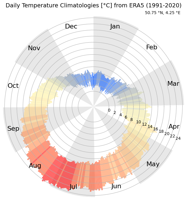
And finally, let’s set up the plot nicely. This can easily be customised, but for now we do something similar to ERA Explorer
latSuffix = 'N' if nearest_lat > 0 else 'S'  # Latitude suffix: 'N' for +ve, 'S' for -ve
lngSuffix = 'E' if nearest_lng > 0 else 'W'  # Longitude suffix: 'E' for +ve, 'W' for -ve

# Abbreviated month names (e.g., Jan, Feb)
month_names = [calendar.month_abbr[i] for i in range(1, 13)]

# Custom color palette for daily polar plot (blue to red gradient)
dailyPolarColors = [
    "#0055ff", "#4376ce", "#859bb4", "#b1bab8", "#d3d7b2",
    "#f2eaa3", "#fff29e", "#fee996", "#fed383", "#ffb369",
    "#ff8949", "#ff4e21", "#ff0000"
]

# Compute cumulative days at the end of each month for a leap year
cumulative_days = cumulative_days_in_months()

# Convert months into angles in radians for polar plotting
angles = np.linspace(0, 2 * np.pi, len(clim), endpoint=False)
angles = np.append(angles, angles[0])  # Close the loop

# Extend daily min and max to close the loop
daily_min = np.append(clim['daily_min'].values, clim['daily_min'].values[0])
daily_max = np.append(clim['daily_max'].values, clim['daily_max'].values[0])
heights = daily_max - daily_min  # Height of bars (temperature range)

# Radial axis limits
ylim0 = min(daily_min) - 5  # Slightly below minimum temperature
ylim1 = max(daily_max)      # Maximum temperature

# Normalize colors based on daily max temperatures
min_of_daily_max = min(daily_max)
cmap = ListedColormap(dailyPolarColors)
norm = BoundaryNorm(
    boundaries=np.linspace(min_of_daily_max - 0.01, ylim1 + 0.01,
                           len(dailyPolarColors) + 1),
    ncolors=len(dailyPolarColors),
    clip=True
)
colors = cmap(norm(np.clip(daily_max, min_of_daily_max, ylim1)))

# Create polar plot
fig, ax = plt.subplots(figsize=(8, 8), subplot_kw={'projection': 'polar'})
ax.set_frame_on(False)
ax.set_theta_direction(-1)  # Clockwise direction
ax.set_ylim(ylim0, ylim1)

# Customize axis ticks
ax.set_xticks([])
ax.set_yticks(range(0, int(max(daily_max)) + 2, 2))

# Shade alternate month segments
for index, nDays in enumerate(cumulative_days):
    previous_nDays = cumulative_days[index - 1] if index > 0 else 0
    width = nDays - previous_nDays
    mid_angle = np.deg2rad(nDays * 360 / 366) - np.pi / 2
    start_angle = mid_angle - np.deg2rad(width / 2)

    ax.text(
        start_angle, 0.9 * ylim1, month_names[index],
        ha='center', va='center', fontsize=16
    )

    if index % 2 == 1:
        continue

    ax.bar(
        x=start_angle, bottom=ylim0, height=ylim1 - ylim0,
        width=2 * np.pi / 12, color='lightgray', alpha=0.5
    )

# Plot temperature bars
bars = ax.bar(
    angles - np.pi / 2, heights, width=2 * np.pi / len(clim),
    bottom=daily_min, color=colors, alpha=0.6,
    label=f'{abs(nearest_lat):.2f} °{latSuffix}, {abs(nearest_lng):.2f} °{lngSuffix}'
)

# Add legend and title
ax.legend(loc='upper right', bbox_to_anchor=(1, 1.05), framealpha=0, handlelength=0)
years = f'{date_range[0][:4]}-{date_range[1][:4]}'
plt.title(
    f'Daily Temperature Climatologies [°C] from ERA5 ({years})\n',
    fontsize=14
)

# Display plot
plt.show()